Computer vision in agriculture

Computer vision has been applied in a broad range of sectors and industries. The most recognisable use cases of computer vision include self-driving cars, the diagnosis of diseases in medicine, and its help within factory automation.

Alongside the industries mentioned above, agriculture has also started incorporating computer vision in its day-to-day operations. Several uses of computer vision in agriculture include the classification of crops, weed detection, automating picking fruits and vegetables, and monitoring fields using drone or satellite imagery.

The subject of this blog post relates to the latter use case. More specifically, we at Superlinear developed a system to detect field boundaries using satellite images. This system is part of a larger project for Yara where we develop, in collaboration with Sentera, an AI screening tool to support farmers in their carbon neutrality journey.

This blog post shows you how to efficiently set up an instance segmentation system, which is a system that detects and delineates each distinct object of interest from an image. More specifically, we’ll discuss implementing a Mask R-CNN model that detects field boundaries using satellite images. Aside from that, we’ll also show you some best practices to get good results fast and what their influence is on the final result. This blog post comes together with a GitHub repo, which you can find here.

Supporting the Agoro Carbon Alliance with Computer Vision

On June 8th 2021, Yara launched the Agoro Carbon Alliance to help support climate-positive practices in agriculture. Superlinear helps Yara in achieving this goal by building machine learning solutions that operate on a field level. These solutions aim to monitor an individual field throughout time and detect several agricultural practices such as tillage, cover crops and others.

To apply machine learning on a field level, it is mandatory to know the field's boundaries. 

Unfortunately, only one single geographical coordinate, expressed in latitude and longitude coordinates, is known for every field of interest. There are already some APIs in place that can do these conversions, but these are relatively expensive. Hence, we implement our own solution using computer vision and satellite data to translate this geographical coordinate into a bounded field.

To detect the field boundaries, we used a state-of-the-art instance segmentation network called Mask Region-based Convolutional Neural Network (Mask R-CNN). We relied on Google Earth Engine for the model inputs, a large catalogue of open-source satellite image and geospatial datasets.

From object detection to instance segmentation

As mentioned above, we used an instance segmentation model to determine a field’s boundaries. But what is instance segmentation exactly? Instance segmentation is a practice within computer vision that tries to localise and classify individual objects while also delineating each specific object from the rest of the image.

Figure 1 shows a high-level description of how instance segmentation works. Summarised into a single sentence, instance segmentation will “first detect then segment”. In other words, it applies object detection first on the input image to recognise, classify, and localise each object of interest. This results in a bounding box around every recognised object, together with a corresponding class label. Afterwards, it applies binary segmentation to every sub-image created by the different bounding boxes. This binary segmentation will separate the foreground (object) from the background, resulting in a cut-out of the object.

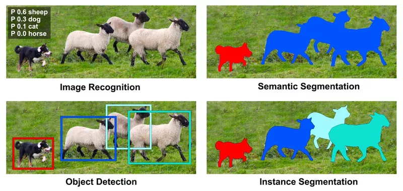
Figure 1: Types of object classification and localisation

Implementing a Mask R-CNN model trained on satellite images

Now we have a high-level idea of how instance segmentation in Computer Vision works, it’s time to implement a model that performs this task. This section addresses the necessary components that we need to implement a solution for our use case.

Mask R-CNN for instance segmentation

To perform instance segmentation, we use the Mask Region-based Convolutional Neural Network (Mask R-CNN) model. Figure 2 shows an abstract diagram of how Mask R-CNN works. On a high level, this model consists of two different parts: a part that creates features for each region of interest, and a part that translates these features into predictions.

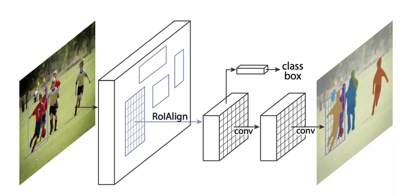
Figure 2: High-level description of Mask R-CNN

The Mask R-CNN starts from a Faster R-CNN model, which is used for object detection. This model uses a single ResNet CNN backbone to extract features from the input image, in parallel with a Region Proposal Network to detect the individual objects in the image. Since a detailed discussion on Faster R-CNN would lead us too far from this blog post's main subject, we will not discuss this further. However, I’ll heavily recommend taking a look at this model yourself for those interested since it gives several fascinating insights on how it improved over the regular R-CNN network.

The second part of the Mask R-CNN utilises these image features that are specific to each region of interest. The model uses these features to classify and segment each of the detected regions. As mentioned before, this segmentation works by creating a binary mask to separate the foreground - this being the object itself - from the background in every bounding box.

The implementation is done in PyTorch, using the Mask R-CNN model found in their torchvision library. On their GitHub, they have a large catalogue of different (vision-related) models and datasets, which you can find here.

Satellite images as model input

Now we’ll know what model to use, it’s time to look at the data. As the model’s inputs, we’ll use the National Agriculture Imagery Program (NAIP). This is an open-source dataset available on Google Earth Engine (GEE). GEE is a large dataset collection that provides satellite imagery and geospatial data covering the whole world. These datasets vary wildly in the spectral range they cover, their resolution, as well as the frequency of the data. This makes that the data GEE captures can be used for a large variety of use cases.

As Figure 3 shows, the main benefit of the NAIP dataset is its high quality: it ensures no interference of clouds in the images, and a 1-meter resolution, which is significantly better than most datasets available on GEE. Even though the NAIP dataset only provides several images per year, this isn’t a problem for our use case since we can safely assume that a field’s boundaries won’t change during a single season.

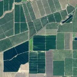
Figure 3: Example NAIP image

There are, however, two main disadvantages of the NAIP dataset. The first disadvantage is that this data is only available in America. This implies that an alternative should be used if one wants to use this model outside of the USA. A second disadvantage is that there are sometimes strides missing in the data. A dirty solution to this problem is to mosaic a previously made image into this stride. However, as Figure 4 shows, this solution is not optimal since these strides remain visible within the image.

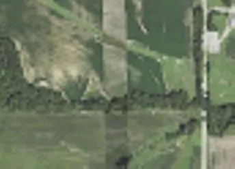
Figure 4: Mosaicing missing stride in data

There exist plenty of alternative datasets as well. For example, if more frequent data or data outside the USA is required, we recommend using the Sentinel-2 dataset. This dataset creates new global images every five days. However, it comes with its limitations as well. First, as Figure 5 shows, the image resolution is now 10 meters, resulting in a notable difference in image quality. Another major downside to this dataset is that clouds are not removed in advance, which tends to interfere with the data on a very frequent basis.

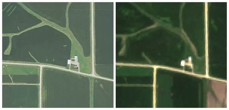
Figure 5: Difference in resolution between NAIP (left) and Sentinel-2 (right)

Other alternative datasets include those that capture the field over spectral bands different from the visible light. Figure 6 shows a visualization of such a dataset. This image is from the Sentinel-1 Synthetic Aperture Radar dataset and shows the change in terrain roughness over the scope of one season. This information is useful since the change in terrain roughness helps to identify certain events such as harvesting or tillage. However, to use this dataset as inputs to our model, one assumes that one field is always harvested/tilled in one day and that neighbouring fields are harvested/tilled on another day, which is not necessarily the case. Another major drawback of using data like this is that there are no pre-trained models to start the training from. This is important since it significantly helps to achieve good results, but more on this in the next section.

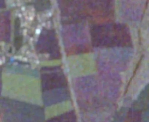
Figure 6: Change in value over one season, obtained by Sentinel-1 SAR

Data annotation

The labels, this being the field boundaries, are created by ourselves since no dataset online would satisfy our needs. Either these datasets operate outside of America, or they didn’t align properly with the NAIP images. To create the annotations for the training- and test set, we use VGG Image Annotator. In total, we labelled 30 images for training and 10 for testing. Figure 7 shows the result of a field together with its labelled mask.

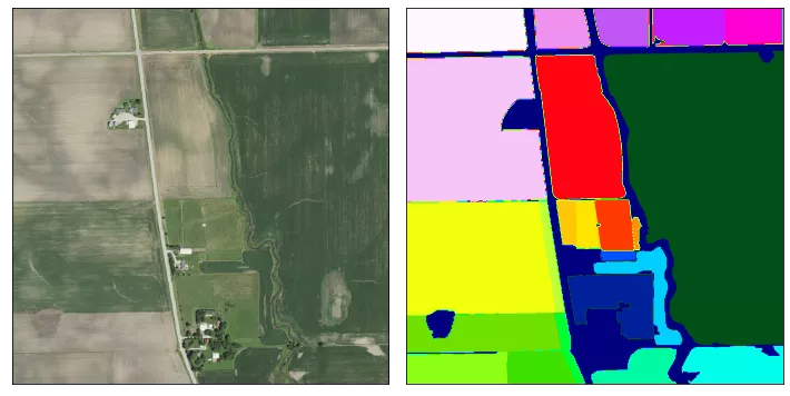
Figure 7: Example of a field (left) with its annotated mask (right)

Get good results fast

To get good results fast, we’ve applied two best practices to train our model. First, we’ll use transfer learning to start the training process with a head start. Secondly, we’ll augment the annotated data to create more training samples.

Transfer learning

We’ll use two pre-trained models in our Mask R-CNN model, both found in the PyTorch model zoo. First, we’ll use a ResNet50 CNN model that acts as a backbone since it transforms the input image into feature vectors of size 4096. These feature vectors are used to predict the bounding box, the class, and the mask of each detected object. Without this backbone, the model needs significantly more data to train.

For the other part of the model, which makes predictions based on the image features, we can use a pre-trained model as well. More specifically, we’ll use a model pre-trained on COCO - the common objects in context - dataset to help with the classification and segmentation. Since the models for this dataset trained over 91 classes, out of which none are “fields”, we replaced the head to fit our needs.

Data augmentation

The second best practice we’ll use to improve performance is data augmentation. Every image in the training dataset undergoes a cut followed by the addition of some noise. During the cut, only a part of the image is used and rescaled to the image’s original size. Noise is then added to this new image, which comes in various forms. Figure 8 shows the original image and four different forms of noise that might be added to the image.

Figure 8: Forms of noise added to the image: (a) original image, (b) rotation, (c) flip, (d) gamma filter to change brightness, and (e) Gaussian filter to add a blurring effect

Influence of model configuration on predictive performance

This section describes the results obtained by our model and its alternative configurations. First, we’ll address what performance metric is used to evaluate the performance. Secondly, different model configurations are assessed together with their performance. At last, we briefly introduce some additional capability our model has and how we exploit this.

Assessing performance using the F1 scoring metric

As this subsection’s title suggests, we use the F1 scoring metric to evaluate model performance. The F1 score, for those not familiar, combines both precision and recall into a single score, as Figure 9 shows.

Figure 9: F1 score formula

To determine precision and recall for a task like this, it is common practice to use a metric called Intersection over Union (IoU). The IoU score of two overlapping regions is equal to their intersection’s surface divided by the surface of their union. In other words, two regions that do not overlap have an IoU score of zero, where two perfectly overlapping regions have an IoU of one. Figure 10 shows how much two regions would overlap given a specific IoU score.

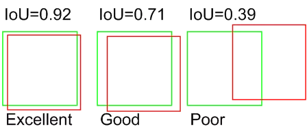
Figure 10: Visual representation of the Intersection over Union score

It is possible to derive a precision and recall score from this IoU by making this score discrete. More specifically, we choose a threshold between zero and one and define a True Positive as an instance where the IoU is greater than this threshold. If the IoU is below this threshold, we define the prediction to be a False Negative. A False Positive is when there is no association between a prediction and a ground truth. Figure 11 shows two examples of this conversion. The final score is the global average of all the obtained scores.

Figure 11: Making the IoU score discrete

From evaluated performance to visual results

Figure 12 shows the evolution of the F1 score over a different number of images that are used during training. As this figure shows, three different model types are trained. A first version - Scratch - starts with only the ResNet50 backbone but without pre-training the remainder of the model on the COCO dataset. Furthermore, it trains on the annotated images as-is, i.e. without the use of data augmentation. A second model - Transfer Learning - has the model pre-trained on the COCO dataset but did not use the augmented data for fine-tuning. The final model - Transfer Learning + Augmentation - uses both a pre-trained model as well as the augmented training data.

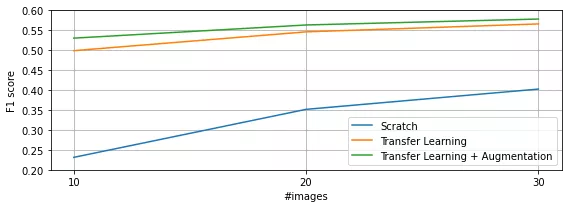
Figure 12: Model results over a different number of training samples

To put these numbers into context, we’ll show you several examples. Figure 13 shows the predictions made by the Scratch model when trained on only 10 samples. This result is rather poor and mispredicts important parts of the image. The worst prediction in this image is that it recognises parts of the forest to be a field. However, it needs to be pointed out that several fields are already correctly classified and bounded in fact. Adding more training data improves the results, although there are still several notable flaws present.

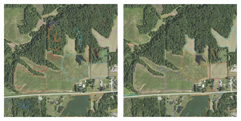
Figure 13: Results of the Scratch model after training on 10 (left) and 30 (right) samples

Figure 14 shows how much improvement one can expect when using a pre-trained model instead of training from scratch while still only using 10 images during training. Most fields are recognised, with decent boundaries for almost all of them. The biggest flaw in this prediction is that one part of the middle field is not recognised. However, this is resolved when training on more images. As seen, more training images also helps improve the quality of the predicted boundaries.

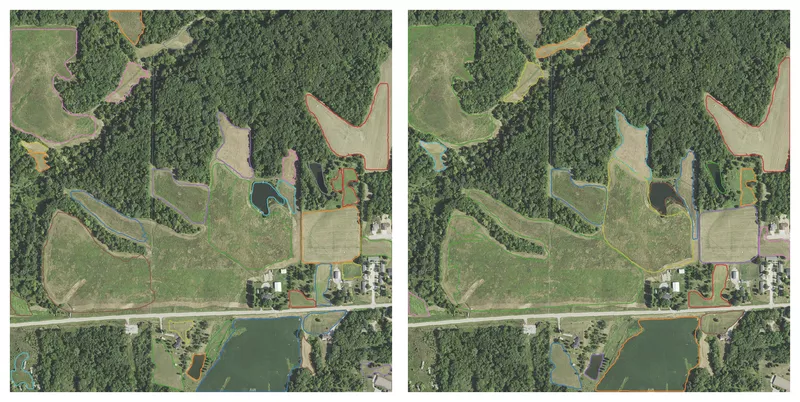
Figure 14: Results of the Transfer Learning model after training on 10 (left) and 30 (right) samples

The addition of augmented training data alongside the usage of pre-trained models mostly improves on the details of the detected field boundaries, as Figure 15 shows. Overall, the model obtains satisfactory results, especially when taken into account that only 30 images are used for training. The only major flaw that the model remains to have is that it is unable to label fields that have an unusual pattern in them, as Figure 15 shows on the right. Luckily, these fields only correspond to a very small fraction of all the fields.

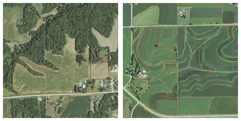
Figure 15: Two results - a good (left) and bad (right) - of the Transfer Learning + Augmentation model after training on 30 samples

Exploiting masking certainty

Since masking works by classifying each pixel within the bounding box to whether or not it belongs to the detected field, it is possible to exploit its classification certainty. By default, a pixel belongs to the field once its predicted score exceeds a threshold of 50%. However, it is possible to change this threshold and only keep the pixels with high certainty. This is beneficial when sampling the field to ensure that you don’t sample points outside the field. Figure 16 shows the change in the predicted boundary for an increased certainty threshold.

Figure 16: Influence of masking certainty: 50% (left) compared to 90% (right)

Further improvements on your Computer Vision model

Before concluding this blog post, we want to first mention some further improvements that might increase the model’s performance even further. There are various changes and additions that might improve performance, ranging from changes in input data to changes in the model itself.

As Figure 12 shows, the accuracy hasn’t fully converged yet. This implies that the addition of more training samples most likely shall increase the model’s performance even further. This increase in performance translates to even more precise field boundaries since the detection of fields is already on point.

Another change to the data that might help the model make better predictions is to use data over other spectral bands than the visible light, as was already mentioned in the “Satellite images as model input” section. However, when using such data, it implies that the pre-trained networks are deemed unusable. Hence, it is mandatory to train these networks ourselves, which requires significantly more training data.

Aside from the input data, it is possible to introduce improvements to the model as well. On the one hand, one could increase the model’s complexity in order to give this model more predictive power. This can be done by using a larger backbone - e.g. a ResNet101 instead of a ResNet50 - or adding more parameters to the classification heads.

A last potential improvement would be to substitute the model entirely. Due to the Mask R-CNN its top-down approach (detect then segment), some weird artifact may occur when bounding boxes are overlapping, as Figure 15 shows. To circumvent this problem, it is possible to implement a bottom-up approach as done in a Spatial Embedding model. This model performs instance segmentation by assigning a class on pixel-level. However, literature shows that these models are often inferior to the detect then segment type of models.

Conclusion

Overall, we’re satisfied with the results obtained by the model. The model can detect most if not all the fields of interest, where most of the detected field boundaries are in line with our predictions. We saw that the fields where the model struggled most are those with an irregular pattern; however, such fields are rather uncommon.

To end with an interesting observation: there is an unexpected but interesting side-effect present in our model’s predictions. As Figure 17 shows, our model is also very capable of detecting and delineating sports fields!

Figure 17: It’s not a bug, it’s a feature